Given the current shortage of data scientists in the U.S. labor market, some argue that employers should simply train internal IT staff to program in a language such as Python or R having strong data-analysis capabilities, and then have these programmers do the company’s data science. Or they may hire analysts with statistical training, but little or no background in optimization. (We discuss this risk in our white paper “Standing up a Data Science Group.”)
This post illustrates an important risk in this homegrown approach to data science. The programmers or statisticians may, in some sense, perform a correct statistical analysis. They may nevertheless fail to arrive at a good solution to an important optimization problem. And it is almost always the optimization problem that the business really cares about. Treating an optimization problem as a purely statistical problem can cost a business millions in lost revenue or cost reductions, in the name of minimizing data science labor expense.
Consider this example. Suppose a company’s marketing department wants to develop a socio-demographic profile of its high-revenue customers. The company could then market to sales prospects having the same profile. Marketing reaches out to IT for help, and IT assigns them a programmer with some statistics training and a little knowledge of R. The marketing department gives the programmer a development data set of 50,000 customer analytic records (CARs), each having 22 independent variables that the marketing department believes might predict revenue per period for a given customer. Marketing instructs the programmer to develop a classification model identifying customers producing annual revenue above a specific target threshold.
Here’s what happens:
- The programmer checks for missing and invalid variable values, replacing them with average values, column by column.
- The programmer creates a new binary variable indicating whether a customer’s revenue per period is above the threshold. It turns out that the threshold identifies the top 1% of customers (by revenue)—in the development data set, 516 high-revenue customers out of 50,000 CARs.
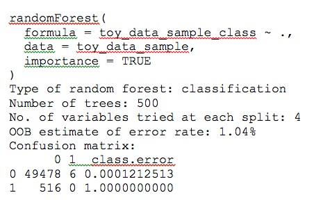
- The programmer uses R’s randomForest library to develop a classification model, and to discover which variables matter most in identifying high-revenue customers.
The programmer is initially delighted to produce a classifier with a 1% error rate; see the (reformatted) randomForest output in Figure 1.
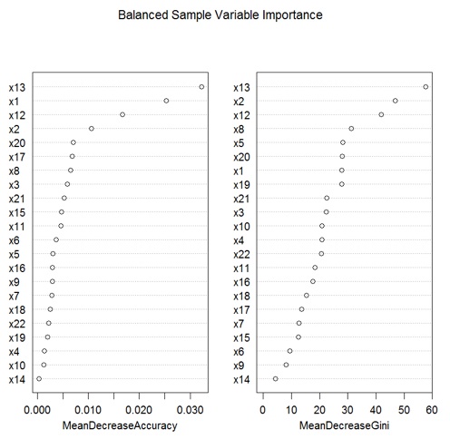
After doing a little more reading, the programmer learns how to generate his model’s importance plots, which suggest that variables x13, x12, and x8 are among the most important in recognizing high-revenue customers; see Figure 2.

The programmer is about to give marketing the good news, when he notices that the confusion matrix is telling him that his classifier never correctly identifies a high-revenue customer. Its misclassification rate for high-revenue customers is 100%!
Some programmers might give up at this point, and tell marketing they’re not really statisticians. Our programmer has more spunk. After thinking for a while, he speculates that the problem is he doesn’t have very many high-revenue customers in his sample. To even things up, the programmer reduces his sample of low-revenue customers to 516, so the sample has equal numbers of high-revenue and low-revenue customers.
The results are strikingly different; see Figure 3.
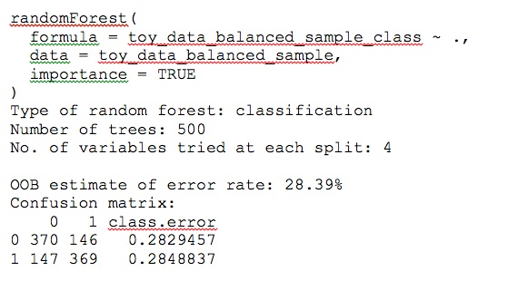
Now the error rate is about 28%, but both classes have the same error rate. Furthermore, the importance plots look different. In particular, where the variable x8 was second in MeanDecreaseAccuracy and fifth in MeanDecreaseGini, now it is seventh and fourth. Clearly it has lost importance (see Figure 4).
What should the programmer do now? Which variables are important enough to use? Is the model at a satisfactory stopping point? How might the programmer improve the classifier’s predictive power? Are the two classes’ error rates equally important? If not, how should the programmer determine their relative importance, and how should he incorporate that into the classifier’s structure? In particular, how does the programmer know whether the classifier will produce the best possible results for marketing?
These are the sorts of questions that a programmer-turned-data-scientist (even with some statistical training) is unlikely to muddle through well. For example, suppose that additional model development could improve the model enough to increase its accuracy from 72% to 90% (for both classes). Suppose the data serviced used by marketing has a database of 100 million names and mailing addresses. Applying the model to the whole population would produce the confusion matrix in Table 1:
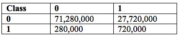
Table 1: Confusion Matrix @ 72% Accuracy for 100 Million Candidates
Marketing only sends ads to candidates in the rightmost column (those identified, incorrectly or correctly, as high-value prospects). So the company would have 27,720,000 + 720,000 = 28,440,000 candidate prospects (a hit rate of 720,000 / 28,440,000 = 2.5%). A typical direct-mail campaign would produce a 1% response rate, or 284,400 respondents. If half of the respondents were high-value, the model would produce 142,200 new low-value customers and as many high-value customers. Assuming further that the company on average breaks even on low-value customers, it would have to mail 28,440,000 prospects to attract 142,200 new high-value customers. If each mailing costs $1, these new high-value customers would have to produce on average $200 in profit (ignoring campaign costs), to cover campaign costs and hence break even. Every dollar per high-value customer beyond that margin would yield $142,200 in profit. And the campaign would have mailed 72% of available high-value prospects, and converted 14% into customers.
At 90% accuracy across both classes, the numbers change somewhat: the model now identifies 10,800,000 prospects, of which 900,000 (12% hit rate) are high value (see Table 2).
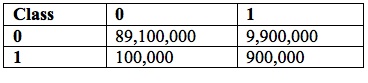
Table 2: Confusion Matrix @ 90% Accuracy for 100 Million Candidates
Under the same assumptions as before, there are 108,000 respondents, 54,000 of them high value. These still must produce $200 in profit for the campaign to break even. Interestingly, every dollar in margin beyond that now only yields $54,000 in profit. The campaign would have mailed 90% of available high-value prospects, but converted only 6% of them into customers. Ironically, the higher-accuracy model would produce less marginal profit and convert fewer total high-value prospects, even though it reached more of them.
Our programmer has learned that sample size matters, at least for some classifiers. And he has arrived at the paradoxical result that higher accuracy across the board may not improve the economic outcome of a direct-mail campaign. In part, that assumption depends on how the proportion of target respondents varies with accuracy. In part, it depends on the relative costs of different error types, and how a model incorporates those costs.
We’ll end the example here, repeating the moral of the story: there is a big difference between analyzing data (in some technical sense) and finding a good solution to an optimization problem. Most data science business problems are optimization problems, not mere data-analysis problems. Optimization requires a skill set far beyond data analysis. Failure to bring that skill set to your data science projects could cost your company millions. Caveat emptor!