Aircraft Trajectory Optimizer

Predictive IoT Services | Problem Definition

In this blog post we examine the use of predictive IoT services and optimization for aircraft trajectory.

The SSN Route Optimizer is a trajectory optimizer that utilizes the Clearable Routes Network (CRN) to find optimized trajectories between an origin point (which may be the aircraft’s current position en route) and a destination. The optimal path is a true 4D path that considers aircraft performance, aircraft category (S/L/H), engine type (P/T/J), and climbs/descents/cruise segments. See Figure 4.

The CRN contains a network representation of the 3-D structure of flight clearances and is created by the cleverly named CRN Generator. The Route Optimizer also relies on the aircraft performance model and a network-based search algorithm such as the A-Star search algorithm. Each is described below, followed by a brief discussion of how everything is pulled together.

CRN Generator

The CRN Generator is a program that acquires and processes large amounts of flight data, then outputs a network with link-specific properties. The input flight data consists of 1) flight meta-data: ID, aircraft type, departure time, origin, destination, etc.; 2) one or more flight/route strings consisting of at least one full route and possibly multiple partial route updates for each flight; and 3) the flight’s trajectory points (4D positions). The current network being tested comes from 30 days of TFM flight data (from 2016-09) and consists of approximately 1.1 million flights.

The flight processing includes a route aggregation stage, a link flight checking stage, and a link building stage. The route aggregation stage creates an aggregated route string created from the initial route string as well as any updates and partial route strings. All airways in the route string are expanded out into their full string of navaids and fixes. The final aggregated route string is a long list of all known fixes and navaids used by the flight.

The flight checking stage makes sure that in addition to the required flight meta-data, the trajectory matches up with the aggregated route. This is done by checking to make sure that both the final route and trajectory vertices and overall lengths are within some tolerance of each other. Also, the profile of the trajectory points is analyzed to make sure that the flight does not start off with a descent, or end with a climb, etc. Any flight that fails the checks is discarded and flights that pass continue on to the link building phase.

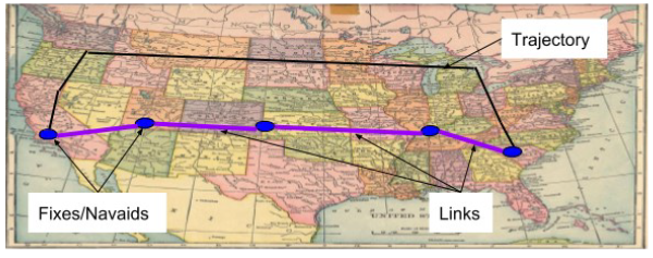
The link-building portion of the CRN Generator uses the aggregated route strings to create sets of links (with the fixes/navaids and altitude ranges as the link endpoints). An example for a single flight is shown in Figure 5. Each link has specific properties computed for it, and then it is stored in a database for use by other programs (like the Route Optimizer). The properties include aircraft type, month of use, climb/descent/cruise information, and an overall usage count. Each property contains a count which is accumulated over all aircraft with that property utilizing the same link. In this way, an overall picture in the form of a network representation is built, representing where and how aircraft are allowed to fly around the NAS.

Predictive IoT Services | Aircraft Performance

The aircraft performance is computed using data lookup tables. Basically, a large amount of aircraft trajectory information is processed to create data tables for each aircraft type. The table below shows a few rows of one of the performance tables.

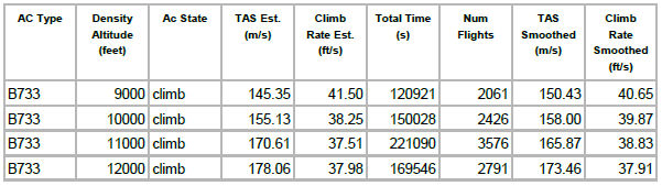
Each table contains the following data: aircraft type, state information (climb, cruise, descent), density altitudes, TAS or true-air-speed, climb/descent rates, smoothed rates, and some other data not used by the performance service. Note that the TAS was computed by using the ground speed and subtracting off wind effects, which were found by looking up the wind data for each flight.

The Performance Generator uses these tables (one for each aircraft / weight / cost index) to compute the time and speed of each segment of a requested partial trajectory (consisting of latitude, longitude, and altitude). Each segment is analyzed to first determine whether or not it is a cruise, climb, or descent segment. Then, using the appropriate state table information, the climb rates (for climb and descent segments) and speeds are computed and provided back for each point in the partial trajectory.

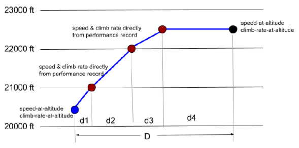
Figure 6 shows an example of how the performance parameters are found for a climb segment going from the initial blue vertex to the upper black vertex. The segment is divided up as it passes through the altitude performance bands defined in the table (one band for each 1,000 feet). The aircraft’s speed and climb rate are then used within each band to determine how much time the aircraft took to pass through each band and how far it traveled. The sum of the distances traveled is then computed and compared to the overall segment length. If the distance traveled during the climb is less than the segment distance, a level/cruise portion is added to the solution. For descent segments, any necessary cruise portion is added to the beginning of the segment solution, rather than to the end.

Predictive Iot Services Model Selection| Dykstra and A-Star Search Algorithms

The Route Optimizer uses the A-Star variant of the Dykstra search algorithm to search the CRN network for the optimal path. For those unfamiliar with Dykstra’s algorithm, it essentially works as follows:

1. Pop the least-cost node from the stack (using the origin node the first time this is performed).
2. If this node is the goal node, then we are done. Simply follow the path back from this current node to all of its parents (which are stored with the node) back to the origin, reverse the path, and you have the least-cost path.
3. Get all possible links coming from this node. In the simplest case, this is all the links emanating from the current node. However, the links are usually tested against one or more constraints and rejected if they don’t pass the test.
4. For the remaining links, compute the cost of traveling the links to the nodes at the other ends and push those nodes and their costs onto the stack.
5. Go back to step 1.

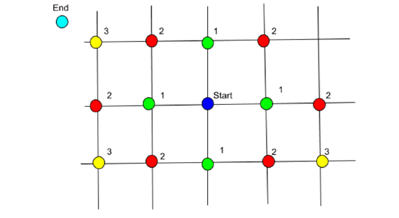
Figure 7 above shows a simple example of a search problem on a grid using distance traveled as the cost for each node. The dark blue node in the center is the starting point, and the cyan colored node in the top left represents the ending node somewhere farther away on the grid. The green nodes are the first nodes found emanating from the starting node, and each of their cost is 1, since they are one unit away from the starting node. For the second iteration, each green node is popped off the stack and the red nodes represent most of the possible nodes stemming from the green nodes. Their cost is 2 since they are two units away from the start. For the third iteration, the yellow nodes represent just a few of the possible steps from the red nodes, and they have a cost of 3.

As you can see, Dykstra’s algorithm tends to spread out in a circular fashion from the origin, and continues until the ‘edge’ of the circle reaches the ending/goal node. Because of this circular behavior, Dykstra’s algorithm builds up a large number of nodes to consider for the solution, and thus memory and computation time can be considerable for some search problems. However, the algorithm does ensure the absolute shortest path between the start and goal, so the basis for using the algorithm is sound. Nevertheless, this process can be improved under many practical circumstances, and this is where the A-Star variant of Dysktra’s algorithm comes into play.

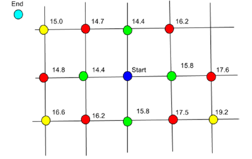
The A-Star algorithm differs from Dykstra’s algorithm only in the calculation of the cost for each node. Instead of simply computing the cost as the cumulative distance from the start node to each path node, it adds in the additional cost of an estimate of the cost-to-go from the node to the end/goal node. This has the effect of making nodes that are closer to the goal cost less than the nodes farther from the goal. The circular shape pattern of the Dykstra algorithm therefore becomes more of an arrow head shaped pattern pointed towards the goal. This means that many fewer nodes are considered and calculated, making the A-Star algorithm more memory and time efficient. It should be noted that given the proper cost-to-go calculation, A-Star is also proven to provide the absolute least-cost (or optimal) solution. The diagram below is a copy of the Dysktra diagram but with the costs computed by the A-Star algorithm. In the example, the starting node is considered to be at 0,0 and the goal is at 10,10.

Putting All These Predictive IoT Services Together

The Route Optimizer puts this all together by finding the “optimal” flight path between an origin and destination node on the CRN using the CRN link properties as constraints to the search, and the aircraft performance calculations for the cost and performance along the links of the search paths.

The A-Star search algorithm is used to search the CRN network and to compute the cost of each node along the network. The current cost for each node is the time of flight from the origin plus the time required to fly from the current node to the end/goal node at fastest possible cruise speed. This link time is computed using the Aircraft Performance library to find the time required to traverse each link given the altitude, climb/descent rate, etc. The extra A-Star cost is simply the distance to the goal divided by the fastest cruise time. The fastest cruise time is used (instead of, for example, the speed at the current node/altitude), to ensure that the final solution path is the optimal (least-cost) path.

The Route Optimizer begins its search by looking for any cruise links and climb links from the starting node. If links with climb properties are found, the algorithm will consider flying to the end nodes of those links with climb altitudes ranging (in steps of 1000 feet) from the current altitude + 1000 feet to the max of the cruise altitude and the top of the climb property. The cruise altitude can also be specified as an upper and lower range for the desired route and once it is reached, the algorithm considers only links with level/cruise properties or climbs/descends within the cruise altitude band (if an upper and lower limit has been provided).

Once the aircraft is over halfway to the goal node, then the algorithm starts searching along links that have descend properties and stops searching along links with climb properties. This is to allow the algorithm to come down and reach the destination. Future iterations of the Route Optimizer will also consider additional constraints using the link properties of aircraft category (sizes of Small, Light, and Heavy), engine type (Prop, Turbo, Jet), weather, winds, and possibly more.

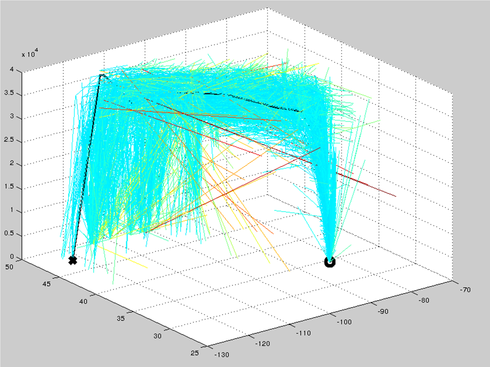
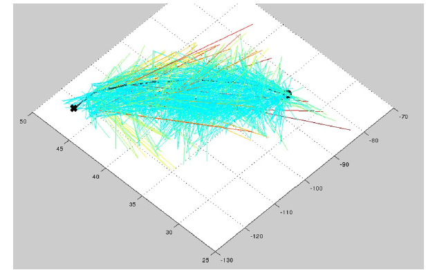
Figure 4 and Figure 8 show the optimal route from KATL to KSEA. The heavy black line (sometimes hidden) is the optimal route. The lighter weight lines are all the links/nodes considered when finding the optimal route, and the redder colors indicate a higher cost. First green, then blue, then cyan show links/nodes with lower and lower costs, respectively. The first figure is a 3D view of the links, and the second figure is a top-down view.

Mosaic can bring these Predictive IoT services to your organization, Contact us Here and mention this blog post.