This is post #2 of a 2-part series focused on reinforcement learning, an AI deployment approach that is growing in popularity. In post #1, we introduce the AI technique, reinforcement learning and the multi-armed bandit problem.
As dedicated readers of our blog will know, at Mosaic Data Science we deploy many flavors of advanced analytics to help our clients derive business value from their data. That being said, as mentioned in a previous blog post (Musings on Deep Learning from a Mosaic Data Scientist), our Air Traffic Management heritage makes us particularly well-suited for AI deployment. In this post I will simulate reinforcement learning by way of its application to a classic problem: the multi-armed bandit problem.
Reinforcement Learning Simulation
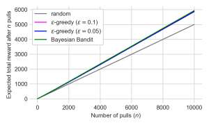
To illustrate these two RL approaches to the MAB problem, I simulated their performance as they interact with a 6-armed bandit. The arm probabilities were set such that 4 of 6 arms had a probability of 0.5, one had a slightly lower probability of 0.4, and the best arm had a slightly higher probability of 0.6. In addition to a Bayesian Bandits policy and two ε-greedy policies with different values of ε (0.05 and 0.1), I implemented a policy that randomly selects an arm to pull. Since the reward achieved each time an arm is pulled is of course random, sometimes an algorithm can perform well just by chance. To help overcome this and estimate the expected performance of each arm, I simulated pulling each arm 10,000 times but starting from scratch 50 independent times. I will report averages over those 50 independent simulations.
The first plot shows the total reward achieved by each policy after 10,000 pulls. The three RL-based policies all perform very well – achieving a total reward close to the maximum 6,000 that would be expected if the best arm were pulled every single time. The random policy performs significantly worse, as expected.
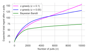
To better see the difference in the performance of the policies, I plotted their average total “regret” after n pulls. Regret is in this case the optimal probability of reward (0.6) minus the probability of the pulled arm. It does not depend on whether a reward was actually received by each pull, so it is less variable than actual rewards. The random policy’s expected total regret is 1,000 after 10,000 pulls (expected regret per pull is 0.1) and it is not plotted to enable a clearer distinction between the other three policies. This expected total regret plot allows us to see that the ε-greedy policy with a higher ε and thus more exploration is able to more quickly identify and exploit the best bandit than the ε-greedy policy with a lower ε.
However, it eventually accumulates more regret than the ε-greedy policy with a lower ε, which is able to more aggressively exploit the best bandit once it has finally learned it. Both of these policies accumulate 60%+ more regret than the Bayesian Bandit, which both learns the best bandit more quickly and also exploits it more dramatically once it is learned. Essentially, the Bayesian Bandit adaptively adjusts its handling of the exploration vs exploitation issue, while the ε-greedy policies are hard-coded to explore less than they should initially and to continue exploring long after it is needed.
Extensions of multi-armed bandits and reinforcement learning
The basic MAB problem and RL algorithms described above only scratch the surface of problems related to MABs or algorithms in the RL family. For example, MAB extensions consider continuous instead of binary rewards, bandit reward probability distributions that vary over time or with other “context” variables, or bandit reward distributions are not independent of each other. Other RL algorithms of course consider the state of the system and how it evolves over time based in part on selected actions, sometimes with the benefit of an existing model of the system but in other cases without. Some RL algorithms can work with a very high-dimensional state (such as deep RL algorithms) or when the state is not known exactly but we only receive noisy observations of it (these are based on Partially Observable Markov Decision Processes). Another fascinating extension of RL known as “inverse” RL attempts to infer the reward function guiding an expert decision-maker, even if they are not always acting optimally with respect to that reward.
Challenges associated with RL & AI deployment
As is implied by the extensions mentioned above, there are a number of significant challenges associated with RL over and above those associated with other types of machine learning. RL and other AI deployment is often data hungry and its development is usually only possible when the environment can be simulated with sufficient accuracy. Even then, training RL algorithms is notoriously difficult, computationally intensive, and challenging to reproduce. While model-free RL approaches exist, RL is generally significantly easier when the system has been well-modeled. Finally, it is not always obvious what the reward and long-term objective based on the reward should be. There may be demonstrations of “good” behavior but no clear specification of a reward function that quantifies how to handle various tradeoffs between competing desiderata.
Closing thoughts
The multi-armed bandit problem and reinforcement learning algorithms can improve performance on real-world problems in which decisions must be made sequentially and under uncertainty. How does your business need to make decisions and learn over time to improve performance? Let us know how we can use data and tools like reinforcement learning to help with AI deployment!


0 Comments