Data Architecture 101, Part 2: Relational Architectures

In our first post we reviewed the rudiments of relational data architecture. This post uses those concepts to survey the main types of relational architectures. These divide fundamentally into two types, the second having four sub-types:

• online transaction processing (OLTP)
• business intelligence (BI)
  • online analytical processing (OLAP) cube
  • data mart
  • (enterprise) data warehouse
  • operational datastore (ODS).

Let’s introduce one more term, before starting our survey. In relational parlance, a schema is a collection of (presumably related) database objects (tables, indexes, etc.). For the rest of this post we’ll assume that all of the database tables for an application reside in a single schema.

OLTP Schemas

OLTP schemas support a transaction-processing application. An application that manages expense reports is an example; each expense report is a separate business transaction. By far the most common operations on an OLTP schema are the CRUD (create, read, update, delete) operations on a single transaction.

Transactions frequently have one-to-many parent/child relations with sub-transactions. For example, one expense report typically has many line items. This gives rise to questions about how you define database transaction boundaries. For example, do you wait for the end user to submit a parent with all of its children before committing the transaction (writing it to disk), or do you commit the parent first and the children later?

The key architectural feature of an OLTP schema is its high level of normalization. Basically, every entity type that is not an atomic data type (does not fit into a single strongly typed column) has its own table. Every such table contains its own surrogate primary key column, and that column has a sequence that generates the key values. In the case of expense reports, that means you could have separate tables for (among other things) employees, addresses, phone numbers, expense reports, expense-report line items, expense-report types, line-item types, cost centers, etc. Naturally a big business would use some of these entity types (logically speaking) across several OLTP applications, so in enterprise-application ERP and CRM suites such as the Oracle eBusiness Suite, OLTP applications may share tables representing common entity types (such as employees and cost centers).

The result of this one-table-per-entity-type rule of thumb is that the entity-relation (E/R) diagrams of OLTP applications contain many arcs (representing foreign-key relations) between the nodes (representing tables). One can often find paths within an OLTP E/R diagram that contain a half-dozen tables. (This makes E/R diagrams more useful for OLTP applications than BI applications, which usually have far simpler join structure.) Thus OLTP SQL statements often join many tables, daisy chaining them with equijoins.[i]

For example, suppose the expense report schema denormalizes the total dollar amount of an expense report’s travel line items, by maintaining the travel total in a column in the expense-report table. Now suppose a user adds a line item to a pre-existing expense report. You would want to update the expense report’s travel-total column in the same database transaction that commits the line item. The wrong way to update the travel total would be to add the new line item’s amount to the existing travel total, if the new line item is a travel item (which assumes the existing total is accurate). The right way would be to recompute the travel total from scratch, something like this[ii]:

update expense_report
set expense_report.total =
(
select sum(line_item.amount)
from
line_item,
line_item_type
where
line_item.expense_report_id = expense_report.id and
line_item.line_item_type_id = line_item_type.id and
line_item_type.name = ‘TRAVEL’ and
expense_report.id = :expenseReportIdIn;

Figure 1: Sample Update Statement

Note that each table joins to just one of the others, equijoining on an ID (surrogate key) column.

The above example illustrates a common way that OLTP transactions are denormalized. Computed values that are frequently used—often, as in this case, because they are attributes of an entity type—are precomputed and stored in the entity type’s table. The example also illustrates how denormalization creates opportunities for data-integrity problems. In this case, some errant application code might insert a travel line item but not update the expense-report table’s travel total, or change a line item’s type to the travel type, without updating the expense report’s travel total. That would make the travel total in the expense report immediately incorrect. If some other application code updates the total the wrong way (as illustrated above), the travel total would also remain incorrect. When you extract data from an OLTP schema, don’t assume that denormalized values are always correct. You’re often better off just extracting the raw data, and computing e.g. aggregates yourself.

Schema normalization is virtuous in OLTP applications because it avoids data-quality problems that arise when an entity is stored in several places. Still, in practice OLTP schemas are not fully normalized; and other kinds of schema features create opportunities for data-quality problems. For example, an application’s design may specify that a combination of two attributes are the natural key for a given entity type, but the schema may fail to enforce uniqueness (or even to require a non-null value) for these columns. Thus, even though a data scientist or extract/transform/load (ETL) developer does not need to design OLTP schemas, these and similar roles need to understand OLTP design enough to spot potential data-quality problems that arise from specific features of an OLTP schema’s design. Understanding OLTP design can also help a data scientist or ETL developer write correct and efficient SQL statements to extract data from an OLTP schema for analysis or transfer into a business intelligence (BI) schema.[iii]

BI Schemas

BI schemas are all designed to support reporting and analysis. The differences among the different types of BI schemas pertain to

• degree of denormalization,
• duration of time for which history is stored,
• breadth of subject matter, and
• whether operational recommendations or decisions depend on (and may be stored in) the schema.

OLAP cube. An OLAP cube is the most denormalized type of BI schema, and is completely denormalized. It contains only values—no surrogate or foreign keys. So a cube is the database analog of a flat file with one record per line, with each record containing only values. If the cube has n columns, each of its rows is an n-tuple, taken from an n-dimensional space of possible values. (Such a space is sometimes called a hypercube or n-cube in mathematics; hence the name.) The virtue of a cube is that it allows fast analytical operations. OLAP tools are optimized to execute these operations on cubes.

Typical analytical operations that OLAP tools execute quickly include the following:

Slicing an OLAP cube fixes a single value for one dimension, while letting all remaining dimensions vary freely, effectively reducing the cube’s dimensionality by one dimension. (In mathematics this operation is termed projection.) For example, one might choose a sales territory or a quarter within a financial year, to examine sales activity within that territory or quarter.

Dicing fixes a single value in multiple dimensions, so it is equivalent to a sequence of slice operations. For example, one might fix both the territory and quarter to view sales activity for the territory in the quarter.

Drilling down starts with an aggregate along one or more dimensions, and chooses a single value for one of the hitherto summarized dimensions, to see the aggregated value at the next finer level of granularity, limited to the newly fixed value. For example, a dashboard might initially present sales by territory for a given financial year. Selecting a single territory might then present a new dashboard presenting sales by city within the territory, for the same financial year.

Drilling up (or, more naturally, rolling up) reverses the drill-down operation by aggregating along a dimension to the next coarser level of granularity. For example, a dashboard displaying sales by city within a given territory for a given financial year might be prompted to roll up sales along the geographic dimension, to produce a new dashboard displaying sales by territory for the same period.

Pivoting replaces one dimension with another, in a given sub-cube (projection) of a higher dimensional cube. For example, one might initially view sales by territory and quarter, and pivot to viewing sales by product and quarter.

These and similar operations make OLAP tools very useful for exploratory data analysis.

A data scientist may use an OLAP cube as a data source for data science tools, as well as using an OLAP tool to explore the data. While cubes are quite close structurally to the sort of data file consumed by data science tools (including R), cubes present several analytical challenges.

1. Cubes rely completely on the ETL process and source systems to ensure data integrity. A cube has no internal features that prevent data-quality problems.
2. A column in a cube may contain order information implicit in the column’s values (names of months, for example). A data scientist might want to encode such implicitly ordered data with numerical values, to expose the order relation to a data science tool. For both reasons a data scientist should avoid assuming that a cube’s data is ready for scientific analysis, and should rather profile[iv] the data to ensure data quality and appropriate representation and typing.
3. OLAP tools and the business analysts who use them can create cubes on the fly by querying the underlying source schema. This means the data in an OLAP cube can have uncertain provenance, currency, lifespan, etc. So, even though a cube is structurally attractive as a data source, a data scientist should be careful not to take the cube’s provenance, currency, or durability for granted.

There are no natural or inherent restrictions on the breadth or time scope of subject matter in an OLAP cube. By definition cubes only support exploration and analysis. They are not appropriate for decision support or decision automation.

Data Mart. A data mart is a schema that captures historical data for a single subject-matter area, such as employee expenses or accounts receivable. The subject-matter area may be narrow or broad, but (by definition) its scope must be markedly narrower than the entire enterprise. Like OLAP cubes, data marts are often the work product of business analysts outside of IT (“shadow IT”). The best structure for a data mart (on a traditional RDBMS such as SQL Server, Oracle, or PostgreSQL) is a star schema, or a collection of star schemas that collectively capture history for a single subject-matter area.

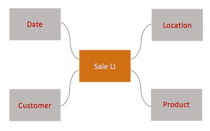
A star schema consists of a central fact table together with a set of dimension tables to which the fact table joins. Basically, a fact tablerepresents a class of business events; each row represents a single event.[v] Each dimension table categorizes the facts in a fact table in a single way. Fact tables also record various measures (quantities) such as date of occurrence, numbers of line items, and price. Occasionally a fact table has no measures; such fact tables are called factless fact tables.

For example, a sales-transaction line item might conceptually be represented by the following 11-tuple:

(date, location, product, customer,
quantity, nominal price, discount rate, discounted price, tax rate, tax amount, total amount)

In a flat file or OLAP cube, each row would contain one of these 11-tuples, with each value expressed literally: dates in a fixed format; locations, products, and customers identified by some natural key (represented as a string); and the remaining values as numbers. In a fact table, the first four values categorize a sales line item, so they become foreign-key columns joining to dimension tables. The measures (in italics) would remain numbers. Figure 2 represents this star schema graphically; Figure 3 contains notional create-table statements for the tables in the star schema.

create table date_dim
(
id integer,
day integer,
month integer,
quarter integer,
year integer
);

create table location_dim
(
id integer,
latitude number,
longitude number,
name varchar2(100)
);

create table customer_dim
(
id integer,
social_security_number integer,
full_name varchar2(100)
);

create table product_dim
(
id integer,
name varchar2(100)
);

create table sales_line_item_fact
(
date_dim_id integer,
location_dim_id integer,
product_dim_id integer,
customer_dim_id integer,
quantity integer,
nominal_price number,
discount_rate number,
discounted_price number,
tax_rate number,
tax_amount number,
total_amount number
);

Figure 3: Notional Create-Table Statements for Sample Star Schema

The table definitions in Figure 3 gloss many technical issues that we’ll discuss in subsequent posts.

Fact tables can have one of three granularities:

Atomic or transaction facts represent an event at a single point in time, such as a single sales transaction at a retail store’s cash register. This sort of fact is usually inserted and never updated or deleted, because the underlying business event occurs all at once.

Periodic snapshot facts represent the state of a periodic measure, such as total sales by month. The current month’s snapshot may be updated at a finer time grain (perhaps daily), until the month is complete, at which point the snapshot is no longer updated (except possibly for accounting corrections). Thus a periodic snapshot aggregates over a single kind of atomic fact, materializing (storing in long-term memory) the results of an aggregation query on the atomic fact table (if it exists). Tables that materialize query results in this fashion are termed materialized views. Historically materialized views have been an important BI performance optimization. The need for materialized views has decreased with the cost of computing power.

Accumulating snapshot facts represent a business process comprised of a well understood sequence of atomic facts. For example, a purchasing requisition may go through an approvals process requiring approvals by a subject-matter expert and a line-of-business manager with adequate signing authority, before being fulfilled. A requisition’s row in an accumulating snapshot fact table would be updated each time an approver approves or rejects the requisition, and finally when the requisition is fulfilled. Thus a periodic snapshot concatenates a sequence of atomic facts, materializing the result of an outer join[vi] over the relevant atomic fact tables (if they exist).

An important best practice in fact-table design is to capture as much detail as possible. This practice is often expressed in terms of granularity, which is a qualitative concept referring to the level of detail with which a database represents a specific entity type. For example, date/time granularity can be months, weeks, days, hours, etc. Transaction granularity can be account, party within account, transaction header (including all of the transaction’s line items), or the individual line item. The imperative is to make your fact tables as fine grained as you can. Your atomic fact table representing transactions should have one row per line item, for example. The reason for this design heuristic is that businesses almost always want to analyze their data at ever finer levels of granularity over time, and one cannot go back in time and capture lost fine-grained history out of a transactional source system (which usually purges data older than the previous calendar or financial year). One implication of this imperative is that you should create atomic fact tables for the facts involved in periodic and accumulating snapshots. These snapshots should be implemented as materialized views.

Relational database tables generally, and fact tables especially, should almost always contain data at a constant grain. Mixed-grain tables are very hard to query correctly, and end users rarely recognize when they are dealing with a mixed-grain table.

Finally, fact tables do not usually have their own surrogate primary key columns. Rather, a fact’s surrogate primary key is its set of dimension foreign keys.

We remarked above that dimension tables categorize facts. Dimensions should never contain measures. They may contain ordinal data. For example, date and time dimensions contain numbers representing and ordering, but not explicitly measuring, time periods. Rather, dimension columns (other than bookkeeping columns such as the surrogate primary key) should contain labels for category values, especially the dimension’s natural primary key. Figure 3 above defines four sample dimensions. Note that the customer dimension includes a customer’s social security number, presumably as that table’s natural primary key. Every dimension must have a natural primary key.

There are several kinds of dimension tables also. In fact, there are several ways to classify dimension tables. Some of these classifications have to do with how you handle

• changes in dimension data,
• hierarchies, and
• small sets of possible values.

We’ll discuss these issues in a subsequent post.

By far the most common query on a star schema selects over the fact table, limiting the active set (set of matching rows) to some constraints on one or more dimensions. Such queries are sometimes termed star joins. For example, Figure 4 contains a query that aggregates total sales, including tax, over all time periods and locations for a given customer:

select sum(sales_line_item_fact.total_amount)
from
sales_line_item_fact,
customer_dim
where
sales_line_item_fact.customer_dim_id = customer_dim.id and
customer_dim.social_security_number = 483241666;

Figure 4: Sample Aggregation Query

The sum() function aggregates over the active set. The first condition in the where clause is the join condition that equijoins the customer dimension’s surrogate key in the fact and dimension tables. The second condition drills down to the specific customer of interest. (In BI parlance conditions like this one that constrain a dimension’s attribute values are sometimes termed filters.) You might spend a few minutes trying to express in SQL the other analytical operations we mention above under “OLAP Cubes.”

There are many technicalities involved in designing a star schema and its ETL so that the data in the star schema has all of the desired data-integrity properties, and so queries against the schema perform well. We will return to these issues in subsequent posts.

There are two structural alternatives to the star schema: snowflaking and third normal form (3NF). Until recently these alternatives resulted in poor performance on most mainstream RDBMS platforms. As hardware becomes more powerful, these alternatives are becoming more tenable. Someday soon we’ll probably see the end of denormalized schemas in BI, because the hardware will support fast querying of normalized transactional schemas. (The first commercial example of this end state is SAP’s Hana platform, which requires powerful current-generation hardware, and which supports a single physical schema for SAP’s transactional and BI applications. As of this document’s writing, Hana has seen very limited adoption.)

A snowflake schema adds a ragged layer of outrigger dimensions to a snowflake schema, to normalize what would otherwise be values in one or more inner dimensions. For example, a product dimension might contain a color attribute. In a star schema, the product dimension would represent color as a string. You could snowflake the color column into an outrigger color dimension table, in which case the product dimension’s color column would become a foreign key referencing the outrigger color dimension. In some cases one inner dimension may snowflake to another inner dimension. If you’re designing a BI schema, think carefully about whether these sorts of relations should be expressed instead within specific fact tables.

3NF schemas are mostly used in BI on shared-nothing massively parallel processing (MPP) relational architectures, notably Teradata. On these hardware platforms 3NF can perform well. It’s interesting that Teradata has remained focused on BI, rather than trying to combine OLTP and BI on a single hardware platform. Outside of the MPP context, 3NF schemas are sometimes used in operational datastores (see below).

(Enterprise) data warehouse. As the breadth of subject-matter in a data mart grows, at some point it becomes more appropriate to call the schema a data warehouse. A data warehouse (DW) must (by definition) contain several star schemas containing at least modestly different subject-matter data. When a DW contains data from most or all of the enterprise, it becomes an enterprise data warehouse (EDW). An EDW supports querying across business functions, while the others do not, making an EDW qualitatively more useful to the enterprise. A query that joins several fact tables from different subject-matter areas is said to drill across the enterprise. Here’s a good example in SQL from the Kimball Group.

A key EDW best practice for supporting drill-across querying is conforming and sharing dimensions. Conforming dimensions means using the same set of values for the same attribute when that attribute appears in several dimensions. For example, a distribution company might have a vehicle dimension specifying maximum vehicle payload in pounds, and also a package dimension specifying package weight in pounds. Sharing dimensions means having a single physical dimension table represent a given logical dimension entity type, and using that table in all fact tables categorizing their events by that logical dimension. The date dimension is the most ubiquitous example of a shared dimension. In short, an EDW is a collection of data marts having conformed and shared dimensions.

Beyond conforming and sharing dimensions, an EDW’s schemas are structurally the same as the schemas of DWs and data marts. The differences lie in the quantity and diversity of data, subject-matter areas, and end users; and in the technical and organizational challenges involved in supporting enterprise-scale BI. These differences are far from trivial. We’ll return to them in subsequent posts. However, a data scientist wanting simply to query an EDW can approach the task with the same query patterns used for data marts and DWs, except for the drill-across operation.

Operational datastore. An operational datastore (ODS) is a data mart or data warehouse that contains historical data used to support some operational activity. Often an ODS is interposed between an OLTP source and a BI database. The following operational activities are common ODS applications:

• reporting for the current operational period (quarter or year)
• ETL
• decision support
• decision automation.

The BI community labels decision support and decision automation, operational BI.

The ODS is of special interest for data scientists and software developers tasked with transforming a prototype data science model into a production decision support system (DSS) or decision automation system (DAS). The DSS or DAS should usually query and write to its own ODS. Thus, the ODS is the type of schema that data scientists are most likely to design.

The main decision is whether to have the ODS schema’s structure (approximately) mirror that of its source OLTP system(s), or that of its destination BI system(s). The deciding factors are, as always, the mix of CRUD and analytical operations the schema must support. Note that an ODS can mix models, using more normalized structure for the tables that support the decision model proper, and more denormalized structure for the historical data that the model analyzes in the course of computing an optimal decision. Few easy generalizations are possible here, and you should be prepared to test thoroughly your ODS schema’s performance with a realistic load, before putting the schema into production.

---

[i] An equijoin matches a single value, often a surrogate key, in two tables.

[ii] This and subsequent sample SQL is Oracle SQL. Each RDBMS vendor roughly complies with “entry level” SQL, but each has significant differences from the others, making it difficult to write platform-independent SQL for all but the most basic operations.

[iii] A subsequent post will catalog common OLTP schema features that lead to data-quality problems.

[iv] There are several open-source tools that aid in profiling, and a few SQL commands can go a long way. We’ll return to profiling relational data in a separate post.

[v] http://www.kimballgroup.com/2008/11/05/fact-tables/ (visited April 5, 2014). The Kimball Group’s Web site is an unsurpassed resource for learning about the practice of BI using traditional relational databases. See http://www.kimballgroup.com/category/fact-table-core-concepts/ (visited April 5, 2014) for a wealth of good advice about fact tables.

[vi] Outer joins basically return empty columns where a source row is missing, allowing for a “partial” join. (Other types of joins don’t return a row when one or more source rows are absent.) We’ll return to join types in a subsequent post.