This is post #1 of a 2-part series focused on reinforcement learning, an AI approach that is growing in popularity. In post #2, we will report on results of a simulation of the two reinforcement learning algorithms introduced here in post #1 and conclude by discussing some extensions and providing thoughts on the types of real-world problems for which reinforcement learning is likely to be appropriate.
As dedicated readers of our blog will know, at Mosaic Data Science we deploy many flavors of advanced analytics to help our clients derive business value from their data. That being said, as mentioned in a previous blog post (Musings on Deep Learning from a Mosaic Data Scientist), our Air Traffic Management heritage makes us particularly well-suited to deploy reinforcement learning advanced analytics techniques. In this post I will provide a gentle introduction to reinforcement learning by way of its application to a classic problem: the multi-armed bandit problem.
Multi-Armed Bandits
In its simplest form, the multi-armed bandit (MAB) problem is as follows: you are faced with N slot machines (i.e., an “N-armed bandit”). When the arm on a machine is pulled, it has some unknown probability of dispensing a unit of reward (e.g., $1). Your task is to pull one arm at a time so as to maximize your total rewards accumulated over time.
While simple, the fundamental issue of exploration versus exploitation makes this problem challenging, interesting, and widely applicable to real-world problems. If a machine dispenses rewards the first five times you pull its arm, should you forget about exploring other machines and just continue to exploit what seems to be an excellent choice? This sort of a decision arises in many contexts where the MAB problem (or its extensions) has been applied, such as internet display advertising, clinical trials, finance, and commenting systems.
Reinforcement Learning
Like supervised and unsupervised learning, reinforcement learning (RL) is a type of machine learning. In supervised learning contexts, each training data point comes with a “ground truth” label or “target variable” to be predicted. In unsupervised learning contexts, we are not provided with such labels or targets but instead asked to identify meaningful patterns or groupings in a data set. In RL contexts, we are presented with an environment and find ourselves in a situation (a “system state”) and are then asked to make a decision or select an action. Selected actions influence transitions to new states. Rather than a ground truth label or target variable, we are presented with rewards (sometimes only occasionally), which are to be accumulated over time. These rewards guide learning without providing example “correct” labels or values, so RL can be classified as a type of semi-supervised learning. The box diagram below depicts the RL context, which is formally known as a Markov Decision Process. The mapping from states to actions used by the agent is often referred to as a “policy.”

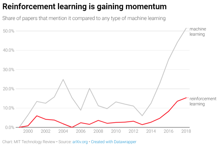
Driven in part by its key role in human-champion-defeating game-playing systems like AlphaGo and AlphaGoZero, RL is climbing towards the peak of a hype cycle near you. As depicted in the graphic below summarizing papers published on arXiv.org (an increasingly popular home for ML and AI research), RL is growing in popularity among researchers, in part driven by extensions of traditional RL that leverage deep neural networks (“deep RL”). More established applications of RL include clinical trials, an alternative to A/B tests, and robotics. Newer (often deep) RL methods have led to applications in areas such as recommendation systems, bidding and online advertising, computer cluster management, traffic light control, and chemistry. More online courses related to RL are hitting the market (e.g., Udacity’s Deep RL nano-degree) and open-source RL environments (e.g., OpenAI Gym) and RL algorithm software are maturing (e.g., Google’s Dopamine, Facebook’s Horizon), making it easier for the masses to try RL.
Using Reinforcement Learning For the Multi-Armed Bandit Problem
To continue the gentle introduction to RL, we’ll briefly describe two RL algorithms for the MAB problem.
Q-learning and ε-greedy policies
One flavor of RL algorithm is called “Q learning,” in which we attempt to learn an estimate of the optimal “state-action value function” Q*(s,a). This function gives the expected future rewards of being in state s and selecting action a, assuming we act optimally in the future. A popular deep RL approach is deep Q networks (DQN), in which a deep neural network is used to estimate Q*(s,a). If we know Q*(s,a) for all s and a, selecting optimal actions is as simple as picking the action a that maximizes Q* for the current state s.
In the MAB problem defined above, we can get away with using a Q(a) that merely estimates the expected reward achieved by pulling a given arm a. One way to estimate that expected reward is by the fraction of pulls of arm a that returned a reward. Rather than acting completely greedily by only selecting the arm with the highest current estimate of Q(a), we can ensure some exploration by, with some probability ε, selecting an arm at random. This mix of greedy and random behavior leads to the name “ε-greedy” for this sort of a Q-learning policy for selecting actions.
Bayesian Bandits policies
Another RL approach that can be applied to the MAB problem is a Bayesian Bandits policy. In this sort of a policy, we model our uncertainty about the probability that each bandit will dispense a reward using a Beta probability distribution. A Beta distribution is not only flexible but also very easy to update as we get new information by observing the result of each pull of a bandit’s arm. Representing uncertainty about the parameters of a probability distribution (in this case a single parameter per arm describing the probability it will dispense a reward) with another probability distribution may be confusing in a way that is reminiscent of the dream levels in the movie “Inception”, but it is an incredibly useful and powerful modeling technique that is fundamental to Bayesian statistics. In this context, we use our uncertainty about these parameters to enable a natural way to balance exploration vs exploitation: we sample from the distribution describing our uncertainty about the probability of a reward for each arm, and then pull the arm that happened to have the largest sample. Since we start with a uniform prior distribution for each arm (suggesting we have no idea whether its probability will be high or low), we are initially equally likely to pick any given arm. After updating the distribution for each arm with Bayes’ rule many times, we eventually become quite confident about which arm is best and are thus very likely to always draw the largest sample from its distribution, leading to very little exploration and almost complete exploitation.
In the second installment of this blog series, Mosaic will simulate both reinforcement learning approaches and report out on the results! Stay tuned.


0 Comments