Why Enterprise Data Warehouse Projects Fail

Summary

Our paper focuses on why enterprise data warehouse projects fail and what to do about it.

Introduction

Everyone knows data warehouses are risky. It is an IT truism that enterprise data warehouse (EDW) projects are unusually risky. One paper on the subject begins, “Data warehouse projects are notoriously difficult to manage, and many of them end in failure.”¹ A book on EDW project management reports that “the most experienced project managers [struggle] with EDW projects,” in part because “estimating on warehouse projects is very difficult [since] each data warehouse project can be so different.”² Many articles about EDW risk cite the laundry lists of EDW failure and risk types in Chapter 4 “Risks” of the same book, arguing that EDW project riskiness derives from the multitude of risk factors inherent in EDW projects. Likewise, experts such as Ralph Kimball offer numerous guidelines for decreasing EDW project risk.³

One risk factor stands out. We agree that EDW projects are complex, and have many risk factors. We also agree that in general, complex projects are more difficult to manage. Having said that, several decades of experience with EDW projects lead us to focus on one particular pattern of EDW project failure that we believe is largely responsible for EDW projects’ reputation for high risk. This white paper describes the failure pattern, explains the risk factor behind the pattern, and suggests how to avoid the risk while delivering value as quickly as possible throughout the project lifespan.

The Failure Pattern

The pattern proper. The failure pattern is surprisingly mundane:

1. The EDW project’s business sponsors agree to fund the project.
2. In exchange for sponsorship, the sponsors pressure the project team to deliver substantial business value early—typically within three months of project onset. More generally, the sponsors require a project roadmap that promises frequent delivery of major new increments of functionality.
3. Eager for a chance to build the EDW, the project team negotiates and commits to a frequent delivery schedule, starting with delivery of some high-visibility data or reports at the end of the first project phase.
4. The project team works very hard through the first project phase, but still does not deliver its initial commitments on time.
5. As time progresses the inevitable frequent scope changes (that partly make EDW projects infamous) accrue. These divert the project team’s attention from its original commitments. The team may renegotiate the delivery schedule, but nevertheless continues to fall ever more behind.
6. Eventually the project’s schedule dilation ruins the project team’s credibility. Management replaces one team of EDW developers with another, management itself gets replaced, or the project is scrapped.

Here’s the remarkable thing about this pattern: even experienced EDW technologists well able to anticipate scope changes find themselves in the same bind. The scope changes per se are not the root of the problem. Nor is the problem just a failure to renegotiate schedule commitments; these renegotiations are a typical part of the pattern. Rather, the problem lies with the project team’s failure to estimate time requirements accurately—even time requirements for re-negotiated priorities—especially in early project phases. The key question is why this occurs. To answer this question, we must detour into data architecture enough to grasp a few of its basic concepts, notably the entity type.

Data Architecture 101. An entity type is a class of things that a database represents. Common business examples of entity types include customer, product, and address. A typical business database represents on the order of 100 entity types.

Data architects organize entity types into data models. A logical data model represents entity types in the abstract. A physical data model realizes a logical model in a given physical database.⁴ In principle, both types of model account for the logical relations among entity types.⁵ However, the data architect must decide which relations a data model actually captures. A good logical model is fairly exhaustive about these relations, but a physical model typically represents a proper subset of those in the logical model.⁶

Precedence relations in logical models. Now, suppose that within an EDW’s logical model, two entity types have some relation. For example, the logical model might represent the customer and purchase-transaction entity types, with each customer optionally making several purchases.^7,8 In such cases one of the entity types must precede the other in two senses, both important to the EDW development process:

Physical-implementation precedence: One entity type’s physical model must be implemented first. Here, the customer (dimension) table can be implemented physically, regardless of the existence of a purchase (fact) table. But the purchase table must have a foreign key referencing the customer (or customer group) dimension table’s surrogate primary key column, to implement fully the physical model of a purchase.⁹

ETL-implementation precedence: One entity type’s extract-transform-load (ETL) process must be implemented first. In our example one could load a customer without having loaded any particular purchase, but one cannot load a specific purchase without first having loaded the customer (or customer group) making the purchase.¹⁰

These two precedence relations always run in the same direction, so logically speaking they can combine into a single precedence relation.

A natural visual representation of the entity-type precedence relations in a logical model is a directed graph, where the arcs (arrows) represent precedence. For example, Figure 1 below represents customer preceding purchase:

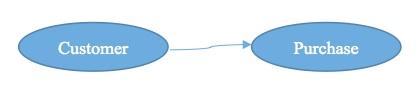
 Let’s call this sort of diagram the logical model’s precedence digraph (PDG).¹¹
A PDG has three interesting properties.

PDGs are acyclic: A PDG is not necessarily connected, but each of its connected components is necessarily acyclic. A cycle would imply that some entity type precedes itself.¹²

PDGs have stages: As is true for any directed acyclic graph, the nodes can be arranged into stages. A node is in stage 0 if it has no predecessors. It is in stage n (for n > 0) if all of its predecessors are lower-numbered stages, and at least one of its predecessors is in stage n – 1. A typical EDW PDG has about 10 stages.¹³

Most of the good stuff is in the high-numbered stages: The entity types most useful to a business generally appear in a PDG’s late (high numbered) stages. For example, analyzing early-stage entity types such as dates, locations, and products does not typically provide much business value per se. In contrast, purchases may involve products, customers, contracts, discounts, locations, dates and times, salespeople, etc. So all of these other entity types must precede purchases in the PDG, forcing the purchase entity type to appear in a late stage. And analyzing purchase patterns is a high-value EDW activity.

Entity-type precedence and EDW project scheduling. We can now explain the failure pattern we describe at the start of this paper, in terms of PDGs. Here are the key insights:

1. EDW project sponsors want to report on and analyze late-stage entity types, early in the project.
2. When EDW project teams promise delivery of late-stage entity types, they habitually fail to recognize that they are also committing to deliver all of the so-far unimplemented entity types required by the promised late-stage entity types. Early in an EDW project, most of a late-stage entity type’s PDG predecessors are unimplemented. So the risk of over-commitment is greatest at project onset.

Notice that the risk is likely to be present each time a project team re-negotiates a project schedule. This is true because the re-negotiation is usually a response to shifting sponsor priorities, not to the project team’s discovering the extent of its over-commitment.

Outside of our own work, we have never seen EDW project teams consider formally how entity type precedence relations bear on project scheduling. In particular, we have never seen an EDW team construct a PDG. Nor to our knowledge has anyone developed and published an EDW project-scheduling methodology based on the PDG.

The Remedy: EDW Project-Schedule Optimization

In our experience the best way to avoid EDW project over-commitment is to maintain a PDG for the EDW’s logical model, and to use the PDG to inform the project’s implementation schedule. In what follows we enlarge this recommendation into a formal model of optimal EDW project scheduling. Some of the model’s elements will be familiar to anyone with EDW experience.

Enterprise ontology. The scheduling model requires an enterprise ontology, which is a logical model that lists each entity type’s data sources (databases, OLTP applications, etc.) with their volumetrics, and that records other metadata relevant to EDW implementation. For technical reasons the ontology should limit itself to entity types that will be represented by a single table in the physical model. For example, a person entity type is too abstract, because an EDW will generally have several tables representing different kinds of people: employees, supplier contacts, customer contacts, etc.

Functional areas. A functional area is a collection of entity types that satisfy the reporting requirements of a given business function. (One entity type may appear in many functional areas.) For example, a product-definition functional area might require four entity types: manufacturer product, supplier product, internally developed product, and unit of measure. This functional area might serve the product-management organization. A typical EDW project will have on the order of 100 functional areas.

Each functional area should list the reports required by the corresponding organization. (Several organizations may require the same report.) Each report should be mapped to the entity types it queries. Each report should also be assigned a utility weight, that is, a dimensionless positive number representing the report’s relative importance to the business. We suggest these weights be integers between one and 10.

Project schedule. A project schedule is a sequence of project stages. Each functional area belongs to exactly one project stage.¹⁴ Consistency with the PDG is a necessary condition for feasibility. More formally, a schedule is infeasible if the following conditions hold:

1. Functional area A precedes functional area B in the schedule.
2. There exist entity types x and y such that x is in A and y is in B.
3. Entity type y is an antecedent of x in the PDG.

A feasible schedule thus traverses the PDG (visits each node once) while visiting a given node only after visiting all of its predecessors. Thus placing a functional area in a given project stage means the team must implement all of the so-far unimplemented entity types required by the functional area, including all of the antecedents required by the functional area’s so-far unimplemented reports, in that project stage.

It is usually desirable to have the project team’s size remain constant over the project lifespan. One can express this naturally by allowing each stage to require at most some fixed number of person hours. If a project team imposes such a load-leveling constraint, it becomes another necessary condition for schedule feasibility.

Workload model. The project team should construct a workload model attributing a number of person hours to implementing each entity type’s physical model and ETL, and to implementing each report. For example, it is common to categorize each data source as having low, medium, or high complexity, and to assume that all source tables having a given complexity level require the same amount of time (same goes for reports).¹⁵ The workload model should also include one-time activities such as hardware and software configuration. The workload model must let the EDW team compute the project’s total and remaining person-hour requirements, given the current project schedule.

Scheduling algorithm. Finally, the model should include a scheduling algorithm. The algorithm must output a feasible project schedule that optimizes remaining project utility. The optimization may be stepwise optimal (greedy) or globally optimal. Ordinarily project priorities (represented by the reports’ utility weights) are likely to change frequently over the project lifespan, so the optimization should be greedy, to ensure the project realizes known high utilities in the short term. Global optimization is only appropriate when all stakeholders are unusually confident that project priorities will not change, which typically implies that all requirements are known and well understood.

It is a practical impossibility for a human to construct a (feasible) project schedule that is near optimal. There are simply too many possible schedules. For example, if a project includes 63 functional areas, there are 63! ≈ 10⁸⁷ permutations to consider (for feasibility and optimality). Fortunately, there is a well-established class of algorithms for solving this kind of problem.¹⁶

Sample results. We have used a greedy algorithm for an EDW project having the following volumetrics:

• 116 entity types
• 372 entity-type precedence relations
• 674 source tables
• 1,267 source-table requirements (for entity tables)
• 325 reports
• 1,380 entity-type requirements (for reports)
• 63 functional areas.

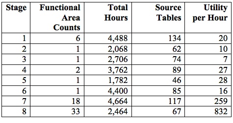
 Setting the work-leveling ceiling to 5,000 person hours yielded a project schedule with 19 stages. Table 1 below lists the stage metrics. The original utilities are between one and 10, but the utility-per-hour figures are scaled up by 10,000 for ease of comparison:

If we consolidate stages 8-19 into a single final stage, preserving functional-area order within the final stage, we end up with an eight-stage schedule. Assuming an eight-person team working 180 person hours per month, the longest stage requires about three calendar months; the shortest, about five weeks. See Table 2:

The business analyst for the same project attempted repeatedly to order the functional areas intuitively. He settled on a schedule that yielded the schedule structure in Table 3:

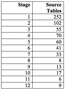
Consolidating the tail to obtain eight stages as before yields the schedule in Table 4:

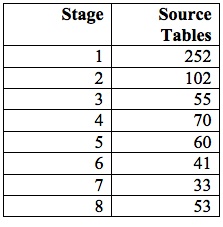
The steady drop in source tables per stage is striking, as is the difference in absolute deviations between consecutive source-table counts. After consolidation, the largest stage of the greedy algorithm’s schedule contains 2.9 times as many source tables as the smallest; but the largest manual stage requires 7.6 times as many source tables as the smallest. See Figure 2 below:

Figure 3 below presents both schedules’ source-table burn rates against an ideal (constant) rate:

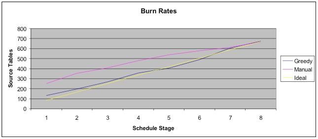
The greedy algorithm achieves far greater load leveling, while choosing at each stage the functional areas that will deliver the most utility possible in an acceptable amount of time.

Using the PDG and scheduling algorithm to negotiate project schedules. The key benefit of using the PDG and scheduling algorithm is not to optimize the project schedule. After all, once the project is complete, the business will probably continue to benefit from the EDW’s data and reports for years, while the project may only last for between six and eighteen months.

Rather, the main benefits are twofold:

• The project team can identify all of the time requirements implicit in a proposed project schedule. This complete understanding of time requirements, together with a realistic load-leveling constraint, lets the project team avoid early over-commitment and the resulting loss of credibility and risk of project failure.
• The project team can use the PDG to help the business sponsors and project team develop a shared understanding of the scheduling constraints that the EDW’s subject matter imposes on the project. This shared understanding can help the business sponsors accept realistic schedule requirements, recognizing that they cannot have everything they want three months after the project starts.

We encourage the project team to print a large copy of the PDG, and use it in schedule negotiations with project sponsors to illustrate scheduling realities by

• circling all of the entity types required by a popular functional area,
• marking the entity types required by some high-utility reports (to illustrate that they tend to lie in the PDG’s late stages), and
• challenging business sponsors to construct a project schedule consistent with the PDG and load-leveling constraint that delivers total utility over the project lifespan comparable to the total utility delivered by the project schedule that the optimization algorithm outputs.

In our experience, this approach quickly persuades business sponsors that they can only get so much so fast. In fact, the approach frees the sponsors and project team alike to change the schedule freely at the end of each project stage, using the algorithm to recompute an optimal schedule after changing report utilities to reflect changing business priorities. Paradoxically, this more formal approach to project scheduling ends up helping the project be as agile as possible, as well as minimizing the risk that the project will miss its schedule.¹⁷

ENDNOTES

1. Robert M. Bruckner, Beate List, and Josef Schiefer, “Risk Management for Data Warehouse Systems.” Lecture Notes in Computer Science Vol. 2114, pp. 219-229 (Springer Verlag, 2001).
2. Sid Adelman and Larissa T. Moss, “Introduction to Data Warehousing,” Data Warehouse Project Management (Pearson, 2000), pp. 1-26.
3. http://www.kimballgroup.com/2009/04/26/eight-guidelines-for-low-risk-enterprise-data-warehousing/, visited January 30, 2014.
4. Logical models are often represented as if they were physical models having one of the normal forms initially defined by the database researchers Codd and Boyce in the 1979s. See http://en.wikipedia.org/wiki/Database_normalization#Normal_forms for the list of normal forms.
5. Data models are similar in principle to class hierarchies in object-oriented programming. Data models differ from class hierarchies in that they do not emphasize the inheritance relation. Object-relational programming attempts to reconcile the relational and object-oriented paradigms, either through a middle tier between application code and database that supposedly eliminates the “impedance mismatch” between them, or through an object-relational database management system that has both relational and object-oriented features. See for example http://www.princeton.edu/~achaney/tmve/wiki100k/docs/Object-relational_database.html.
6. In a physical model, most relations among entity types appear as foreign keys. Here’s the short course on database keys. A primary key is a unique identifier for an entity, that is, an instance of an entity type. A natural primary key is a unique identifier that comes from outside of a database. (Someone enters it manually, or a data-integration process imports it.) A surrogate primary key is a primary key generated by the database, usually an integer. A foreign key is a reference in one table to a surrogate primary key in another table.
7. If several customers can make one purchase together, the relation between customer and purchase is many (customers) to many (purchases); if not, it is one (customer) to many (purchases). Likewise, if a customer need not have a purchase, the relation is optional on the customer side; otherwise it is required. These aspects of a logical relation are termed the relation’s cardinality.
8. In the present example a customer would probably be a dimension, and a purchase a fact, in the EDW’s physical model. The analysis applies regardless, but is more subtle, in other cases—for example, if both entity types are dimensions, or if one is a dimension and the other is an attribute of the dimension. For brevity’s sake we gloss this distinction.
9. Partial representations can skirt the problem at the cost of creating substantial technical debt. Hard experience has taught us to implement an entire entity type’s physical model all at once (and likewise an entity type’s entire ETL process, at least for a given source or set of sources). We have never found implementing partial physical entity types worth the cost.
10. It is possible to load missing dimension data after a fact is loaded, using a design pattern termed a late-arriving dimension. See http://www.kimballgroup.com/data-warehouse-business-intelligence-resources/kimball-techniques/dimensional-modeling-techniques/late-arriving-dimension/. Late-arriving dimensions don’t really avoid the issue, because even when one uses late-arriving dimensions, one still must implement ETL to load the dimension foreign key for the fact whenever the foreign key’s value is available. In a strong sense, late-arriving dimensions are a workaround for a data-quality or data-governance problem. They are not the dimension’s happy-path ETL process.
11. You don’t need to generate the graph manually. Instead, use the open-source utility graphviz to translate a text file listing the graphs nodes and arcs into a nicely formatted graph that you can print in any size.
12. Graphing a logical model’s PDG and checking it for cycles is a great way to discover structural problems in the logical model. The Unix/Linux tsort (topological sort) utility makes checking for cycles trivial.
13. Batch ETL can be architected according to these stages. The data is loaded one stage at a time, and all entity types in a given stage can be loaded in parallel. This approach provably maximizes the parallelism in the ETL process, which is another good reason to construct and study the PDG of an EDW’s logical model.
14. We could define a project schedule more directly as a sequence of entity types and reports. Our definition in terms of project stages means we search a subset of the set of all possible sequences of entity types and reports. As a result, an optimal project schedule may not optimize over this larger set. However, the optimization algorithm is free to optimize the ordering of previously unimplemented entity types and reports within a given stage’s functional areas. So depending on the load-leveling constraint, our definition may not strongly constrain the search. We choose the definition based on project stages and functional areas because the business world generally requires that EDW projects be structured in this fashion, with a stage typically lasting between three weeks and three months.
15. For source tables, we suggest using as a complexity metric the product of column count and base-10 log of row count. The assumption is that replication effort is linear in the number of columns, while data-cleansing effort increases very sub-linearly with record quantity. Then one can categorize a source table as low, medium, or high complexity according to the metric’s value. We likewise suggest a report-complexity metric linear in the number of entity types the report queries.
16. That is, a network optimization problem with path-dependent utilities and costs. See for example Dimitri P. Bertsekas, Network Optimization: Continuous and Discrete Models (Athena Scientific, 1998).
17. In particular, it becomes natural to treat a project phase as an agile/scrum iteration.

---

Copyright © Mosaic Data Science | Data Science Consulting. All rights reserved.