Summary
Applying statistical inference is a great way for businesses to get more value out of there email marketing programs.

Take Our Content to Go
Introduction
A/B testing has been around for a while. Its beginnings can be traced back to agricultural experiments that would test which variation of crops would grow better under specified conditions. Variations of what we now call A/B testing are used in multiple fields such as manufacturing, clinical trials, web analytics and, of course, marketing. In its most basic form, A/B testing compares two versions of something and determines which one results in a more desirable outcome based on a chosen metric. Many data scientists regularly use A/B testing. The advanced statistics involved merely tell us whether or not we can believe that the difference between the metric obtained from each variation is ‘real’ or just due to randomness.
Where to Start with Advanced Statistics
To begin an A/B test we need two things:
- A question or hypothesis to test
- A metric on which the results of the test will be based
The question usually takes the form of: Will applying a change to the subject change (increase or decrease) the metric? The metric can be anything specific and measurable, such as the probability of an individual opening an e-mail or number of webpage views. Let’s go through an example.
I have an e-mail that I want to send out for marketing purposes. There are two subject line variations of that e-mail, and I’m not sure which one will result in a higher probability of opening.
Our question could be: Does Variation A lead to a higher likely that a recipient will open the email than Variation B? We’ll answer that question by looking at the metric probability of opening. To get an idea of how we can analyze the results, let’s show some numbers. Suppose we send out emails to 1,919 recipients with the following results:
| Opened | Not Opened | |
| Variation A | 103 | 873 |
| Variation B | 88 | 855 |
Importantly, the set of sample recipients receiving each variation of the subject line were chosen randomly, so we expect each sample to be good representation of the full population of possible recipients. The observed (“empirical”) probabilities are:
Variation A: 103/(103+873) = 10.55%
Variation B: 88/(88+855) = 9.33%
So, Variation A is better, right? About 13% better! Send out Variation A e-mails!
Actually, we are not sure yet. Here’s where advanced statistics comes in.
In our experiment, we only tested the email on a small subset of possible recipients. We haven’t tested it on everyone we want to send the e-mail to. We cannot be certain that those recipients who haven’t yet received the e-mail will respond in exactly the same way as those that have. What we have is a sample of the population. How do we analyze our sample so that we have a better idea of the overall results? We need a probability distribution for our metric on which to base our analysis so that we can account for possible sampling error – the possibility that the results from our sample test are not representative of how the full set of recipients will respond.
Without going into too much detail, the number of recipients that open an email can be represented by the binomial distribution since there are only 2 types of outcomes possible for an individual recipient: open or not open. In addition, when the number of recipients is large enough, the binomial distribution can be approximated by the normal distribution (bell curve). Lucky for us, the difference between two values represented by normal distributions also follows a normal distribution. So we can calculate confidence intervals around the difference in probability of opening between recipients of the two variations based on the properties of the normal distribution.
This is one of the simpler ways to calculate whether or not the observed difference between variations within the test sample is likely to indicate a ‘real’ difference that would generalize to all possible recipients. Here’s what we need to do:
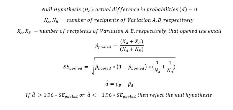
While a thorough explanation of advanced statistics theory is beyond the scope of this whitepaper, let’s hit the highlights.
Our null hypothesis ( ), the thing we are trying to disprove, is that the difference in the opening probabilities between the two groups of recipients is zero – i.e., the two probabilities are the same. The pooled probability ( ) is 0.0995 (9.95%). The pooled standard error ( ) is 0.0137. The observed difference in probabilities ( ) is -0.0122. To test the hypothesis, we multiply 1.96 by and -1.96 by , which results in 0.0268 and -0.0268. We will evaluate this test at a 95% level of confidence. The threshold values +/-1.96 come from the Z-score (since we’re assuming a normal distribution for the actual difference in probabilities) corresponding to this confidence level.
Is -0.0122 > 0.0268? No.
Is -0.0122 < -0.0268? No.
Therefore, we cannot reject the null hypothesis that the two probabilities are equal. What we are saying here is that even though there is a difference in the two probabilities, given the size of our sample, we cannot say with confidence that this indicates a true difference between the two opening probabilities. In statistical terms, we say that the difference is not statistically significant.
Send out Email Variation A or B, it doesn’t matter!
It would be nice if it were that simple. But there are some matters that we glossed over and some that we didn’t even mention.
- If we had more data (larger test samples), would that change the conclusion?
- Would our conclusion change if we chose a different confidence level than 95%?
- Even if a larger test could demonstrate statistical significance, is a difference in probabilities of 0.0122 practically significant from a business perspective?
- Are there ways of segmenting the data that would lead to different results?
- Can I design the experiment better?
The answer to the first two questions are “Yes, it could.” But we’d have to collect more data or do the calculation with different significance levels.
Question three brings up the difference between statistical significance and effect size. For example, a difference in probabilities could be statistically significant – i.e., we believe that the difference observed between the samples is not simply due to randomness – but not be large enough to impact business outcomes. Whether or not a result is practically significant usually is determined by the business. Is a 1% increase enough? Or a 5% increase? Is the cost to implement a change based on the test results more than what will be gained from the change? It will depend on the context. Ideally, we choose a value for practical significance with the business and analyze the data to determine whether the difference is statistically and practically significant.
We will return to question four later in this post.
Question five’s answer is usually “yes.” This question relates to effect size and the statistical concept of sensitivity, and with them we can answer the question “How large a sample do we need to get a statistically significant result if there is a practical difference between the probabilities?” We don’t want to run experiments any longer than we need to, but we want to make sure we run it long enough to detect practically significant differences. Effect size and sensitivity (sometimes also referred to as power) have an inverse relationship, meaning that the smaller the effect size that we want to detect at a particular confidence level, the larger the sample size we will need. This is where the area of Design of Experiments comes into play.
Designing a Better Experiment
First, we will need some basic statistical terminology to discuss this subject.
α (significance) = probability of rejecting the null hypothesis when the null is true (type I error)
1 – α (confidence) = probability of correctly failing to reject the null hypothesis when the null is true (true negative)
β = probability of failing to reject the null hypothesis when the null is false (type II error)
1 – β (sensitivity) = probability of correctly rejecting the null hypothesis when the null is false (true positive)
What we want to determine here is the minimum sample size (e.g., email recipients) necessary to detect a statistically significant result at the desired confidence level and with the desired sensitivity. Detailed mathematics behind this calculation are beyond the scope of this whitepaper. In fact, it’s probably best to search for an online sample size calculator and experiment with it. In any case, we can get some intuition behind that math. To calculate the minimum sample size for the test, we need:
- A ‘baseline’ estimated pooled probability of a user opening an email
- Minimum detectable effect size
- Desired test sensitivity
- Significance/confidence level for determining statistical significance
How do the choices of these values impact the minimum sample size required? The minimum sample size increases if…
- …the baseline probability estimate moves closer to 50%
- …the minimum detectable effect size decreases
- …the desired sensitivity increases
- …the selected confidence level increases (or, equivalently, the significance decreases)
There is an interplay between all of these; however, we can generally say that nothing comes for free – to detect a smaller effect size, increase the test sensitivity, or increase the confidence in the outcome, you’ll need to collect a larger sample. As a quick example, let’s assume our baseline probability is 10%, the minimum effect size that is relevant to the business is +/-3%, our desired sensitivity level is 0.2, and our desired significance level is 0.1. This would mean that we need about 1,290 samples in each variation.
A Real-World Example
Like most businesses, Mosaic Data Science employs e-mail marketing to obtain new clients. We use advanced statistics to optimize these campaigns, primarily using variants of A/B testing. A recent example of the analysis of these campaigns looked at the difference in probability of opening two variations of an e-mail. One of the e-mail templates and associated messaging is focused on ‘what’ Mosaic does, and the other focuses on ‘why.’ The overall goal of this test was to see which template is more likely to be opened by a recipient. The testing of these emails would impact future e-mail marketing messaging.
This advanced statistics analysis is segmented by Industry, which, as you can see in the chart, results in interesting conclusions. Note that this analysis is more complex than the above examples that we discussed earlier; however the basic understanding will aid in being able to read the results properly. The first chart shows the overall difference between the “what” and “why” variations, and the second chart shows the difference segmented by industry.
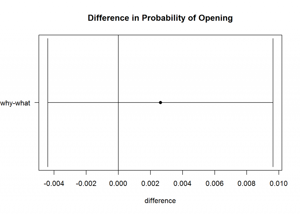
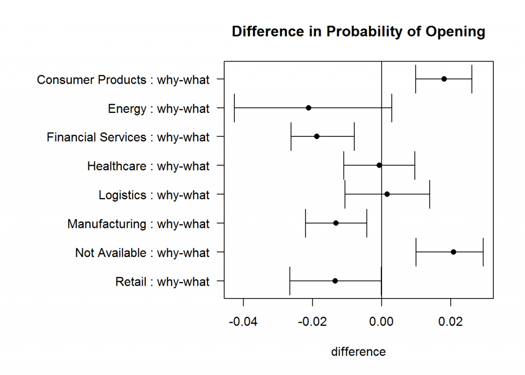
The dots in the chart are the point estimate for the difference in probability of opening, and the horizontal line represents the confidence interval around that average. If the confidence bands include zero, there is no statistically significant difference between the open rates of the two messages. Overall, there is no statistical difference; however, certain industries seem to prefer different variations to the e-mail whereas others show no difference. This highlights the fact that even if the overall difference is non-significant, segments of the sample may be (see question four above). These insights on how certain industries respond to different messages is extremely valuable to our marketing manager. He is able to inform future messaging decisions based on results from these tests.
Testing significance across multiple population segments, however, increases the risk of false positive results and requires additional consideration. This is the realm of multiple hypothesis testing, which we will save for a future whitepaper – or you can contact Mosaic’s data science consultants to help you create a repeatable and reliable test strategy for your marketing campaigns.
Conclusion
What we have covered here only scratches the surface of what can be done with A/B testing. There are many ways of optimizing experimental design, especially if multiple variations need to be tested. In addition, there are many methods of analyzing the results such as Bayesian A/B testing and sequential A/B testing. By applying rigorous advanced statistics to e-mail marketing campaigns, marketing managers can uncover hidden insights informative to increasing clicks, conversions and revenue.


